
An Empirical Analysis Packing Discriminators in Generative Adversarial Networks
The following was originally written in December 2018 as a final project for my undergraduate machine learning course. Additions and clarifications have been made while transfering the report over from LaTex.
Generative Adversarial Networks (GANs) [Goodfellow14] are a family of generative models that have had recent success in generating samples from complex distributions. GANs have been used to produce realistic text, numerical and image samples effectively however they generally encounter a common issue where the model produces samples with little diversity. This problem is referred to as mode collapse and a significant amount of work has been put into finding techniques to alleviate this issue. One of these proposed techniques is a simple extension to the discriminator architecture called packing [Lin18] where the network is trained to validate against multiple samples jointly.
In this report we be performing an empirical analysis on packing to better understand how it works in GAN training. We test networks with and without a packing discriminator on synthetic datasets where mode collapse can be easily be monitored and distribution statistics can be changed to observe how effective packing is under different settings.
Preliminaries
Mode Collapse in GANs:
Mode collapse is a phenomenon in GANs where the generator produces samples that lack the same diversity as the target distribution. More specifically, mode collapse is when the generator’s learned distribution assigns a significantly smaller probability density around the region of a mode compared to that of the target distribution [Lin18]. Mode collapse occurs when the generator becomes so overconfident in certain samples fooling the discriminator that instead of exploring the rest of the data manifold for undiscovered modes, the generator continues to produce similar samples to minimize its loss function.
An example of mode collapse happens while training on the MNIST dataset which has the 10 digits (0-9) as its modes. Using a standard GAN architecture, the model often fails to generate all of the digits, only discovering a few of the distribution’s modes no matter how long the network trains.
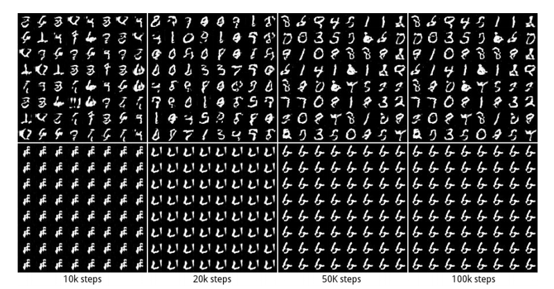
Figure 0: A GAN encountering mode collapse (bottom) vs one that is not (top) [Cho18]
Several approaches have been proposed to deal with mode collapse. These approaches include label smoothing, different loss functions, mixing multiple GANs together and using batch statistics during validation. While many of these techniques have shown to be effective, there is little understanding as to why certain techniques work and which are the most suitable for different cases.
Packing:
Packing is an extension to the standard GAN architecture where the discriminator labels multiple samples jointly to a single real/fake label. The same general network architecture and loss function are maintained from the standard GAN however the discriminator is modified from a network that maps a single input $x$ to a binary label, $D:x \rightarrow \{ 0,1 \}$, into a packing discriminator which maps $m$ inputs $x_1, x_2, …, x_m$ to a single joint binary label, $D:x_1, x_2, …, x_m \rightarrow \{ 0,1 \}$. We refer to $m$ as the degree of packing and the $m$ samples are drawn independently from the real distribution $P$ and the generator distribution $Q$ while training the discriminator.
In a standard GAN, the network can be thought as learning a distribution $Q$ which minimizes the distance between itself and the real distribution $P$, $\min d(P,Q)$. When using packing, the discriminator is given samples from the product distribution of degree $m$ which changes the optimization problem to $ \min d(P^m, Q^m)$. Exposing the discriminator to the product distribution allows for it to better detect the presence of diversity (or lack there of) in generated examples enforcing the generator to explore a wider area of the data manifold and avoid missing modes.
Packing introduces little added computation, going from $\mathcal{O}(wrg^2)$ per minibatch update in a standard GAN to $\mathcal{O}((w+m)rg^2)$ in a GAN using packing of degree $m$ where $w$ is the number of fully connected layers, $g$ is the number of nodes per layer and $r$ is the minibatch size [Lin18].
Experiments
Setup
To analyze the effects of using a packing discriminator, we compare networks with and without packing across different variations of our baseline dataset. The dataset is a 2-dimensional multivariate Gaussian distribution $\mathcal{N}(\mu, \Sigma)$ with 25 means at $(-4+2i, -4+2j)$ for $i,j \in \{0,1,2,3,4\}$, each with $\Sigma=0.0025 \cdot \mathcal{I}$ (seen in the leftmost plot of Figure 1). Experiments are done on variations of the baseline dataset with different variances, mode concentrations and arrangements.
All of the networks use the same generator and discriminator architectures which can be seen in Table 1.
| Generator | Discriminator |
|---|---|
| $z \in \mathcal{R}^{2} \sim \mathcal{N}(0, \mathcal{I})$ | $x_1, x_2, … , x_m \in \mathcal{R}^{2}$ |
| $Dense(2 \rightarrow 400)$, BN, ReLU | $Linear(2 \cdot m \rightarrow 200)$, LinearMaxOut(5) |
| $Dense(400 \rightarrow 400)$, BN, ReLU | $Dense(200 \rightarrow 200)$, LinearMaxOut(5) |
| $Dense(400 \rightarrow 400)$, BN, ReLU | $Dense(200 \rightarrow 200)$, LinearMaxOut(5) |
| $Dense(400 \rightarrow 400)$, BN, ReLU | $Dense(200 \rightarrow 1)$, Sigmoid |
| $Dense(400 \rightarrow 2)$, BN, Linear |
Table 1: Generator and discriminator architectures
The discriminator uses LinearMaxout [Goodfellow13] with 5 maxout units as its activation function. The generator and discriminator both use the standard GAN loss function from [Goodfellow14]. The synthetic training dataset has 100,000 samples that the networks are trained on for 100 epochs using Adam [Kingma14] with equal updates on the generator and discriminator. All other parameters can be found in Table 2.
| Learning Rate = 0.0001 |
| $\beta_1$ = 0.8 |
| $\beta_2$ = 0.999 |
| batch size = 100 |
Table 2: Additonal hyper-parameters
During the experiments we monitor how many modes the generator learns over time. For multivariate Gaussian distributions, a mode exists at each of the distribution’s means and we consider that a mode is lost if no sample within 3 standard deviations of the center of a mode is generated during testing. Other metrics measured are the number of epochs it takes the network to learn all the modes, the proportion of generated samples within 3 standard deviations of a mode (% high-quality samples) and the Jensen-Shannon divergence (JSD) between the target and learned distributions. All metrics are calculated from 2500 samples generated after each epoch.
The dataset, hyper-parameters and metrics closely follow those from the 2D-grid experiment in [Lin18].
Results
The first set of experiments examine the effects of packing on data with different levels of noise applied to it which is simulated by increasing the variance of our baseline target distribution. On the noise-free baseline distribution (Figure 1 and Table 3), the network is only capable of generating 19 of the target distribution’s modes when using a standard discriminator however by adding packing the network learns all 25 modes at $m=3$.
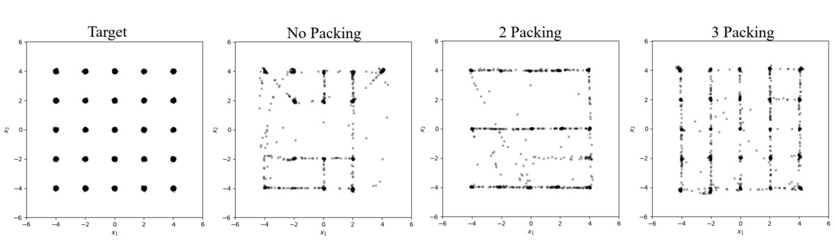
Figure 1: Samples from a 25 mode distribution with $\Sigma=0.0025 \cdot \mathcal{I}$
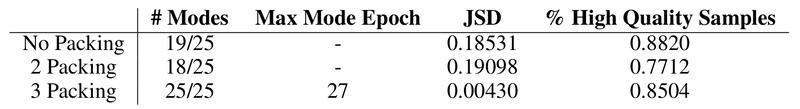
Table 3: Results from Figure 1
When noise is added to the distribution the severity of mode collapse decreases with the standard GAN, recovering 23 modes when $\Sigma=0.01 \cdot \mathcal{I}$ (Figure 2 and Table 4) and all 25 when $\Sigma=0.1 \cdot \mathcal{I}$ (Figure 3 and Table 5). Applying noise to the inputs of the discriminator is a technique that has been explored before [Salimans16, Arjovsky17] and is understood to help smooth the target distribution’s probability mass. In our experiments, applying noise increase the area in the data manifold where the training data lies making the discriminator less strict and allowing the generator to explore without being penalized as severely.
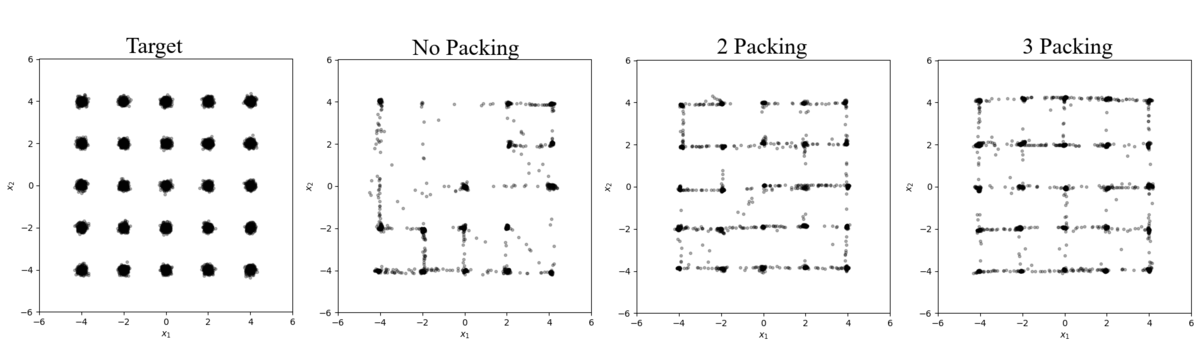
Figure 2: Samples from a 25 mode distribution with $\Sigma=0.01 \cdot \mathcal{I}$

Table 4: Results from Figure 2
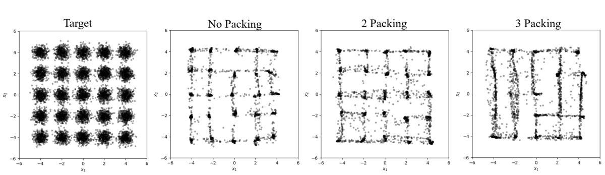
Figure 3: Samples from a 25 mode distribution with $\Sigma=0.1 \cdot \mathcal{I}$
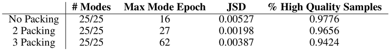
Table 5: Results from Figure 3
The other experiments looked at how the complexity of the distribution impacts the effectiveness of packing. On a low complexity distribution with 9 modes and $\Sigma = 0.0025 \cdot \mathcal{I}$ (Figure 4 and Table 6), the standard GAN can only produce 8 modes after 100 epochs however when packing with $m=2$ is added, remaining the network quickly discovers all 9 in just 3 epochs. This observation shows that the non-packing network quickly converges to 8 of the modes and then stops exploring to prioritize improving the quality of the samples for the modes it has already discovered. When packing is added this bottleneck is bypassed immediately and the network discovers the final center mode.
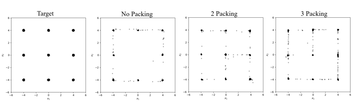
Figure 4: Samples from a 9 mode distribution with $\Sigma=0.0025 \cdot \mathcal{I}$
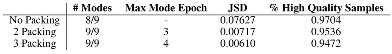
Table 6: Results from Figure 4
On a high complexity distribution with 81 modes and $\Sigma = 0.0025 \cdot \mathcal{I}$ (Figure 5 and Table 7), none of the three networks are able to discover all modes. No packing and packing with $m=2$ discover 59 and 58 modes respectively however we do see $m=3$ significantly outperforming the others discovering 69 of the 81 modes. The architecture used in the experiment is clearly not deep enough to adequately learn this complex distribution however we can still observe from the experiments that adding packing can reduce the degree of mode collapse even in shallow networks.
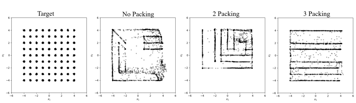
Figure 5: Samples from a 81 mode distribution with $\Sigma=0.0025 \cdot \mathcal{I}$
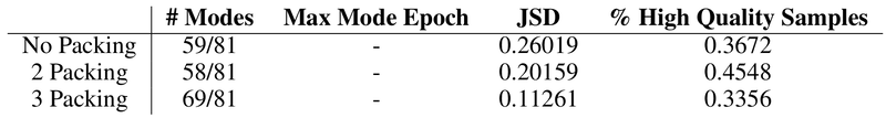
Table 7: Results from Figure 5
To see if the distances between modes impacts how the network explores the data manifold we perform the last experiment on a baseline distribution with randomly spaced modes (Figure 6 and Table 8). All three networks were unable to discover all 23 modes (two pairs of modes combined during the random shuffling) with them each producing the same 20-21. From the plots in Figure 6, we can see that each network failed to discover the same 3 modes in the center-left region of the data manifold. These modes have a relatively larger distance to its neighbours compared to the rest which caused the network to not explore far away from the modes it had already discovered and find the remaining modes. This observation shows that GANs can become biased in its learning, focusing on exploring regions of the manifold that have a high likelihood of generating samples that will fool the discriminator and fails to explore the low likelihood region, where new modes can be discovered, even when packing is being used. How the target distribution is modeled highly influences the generator’s susceptibility to mode collapse and could be important to consider in future work.
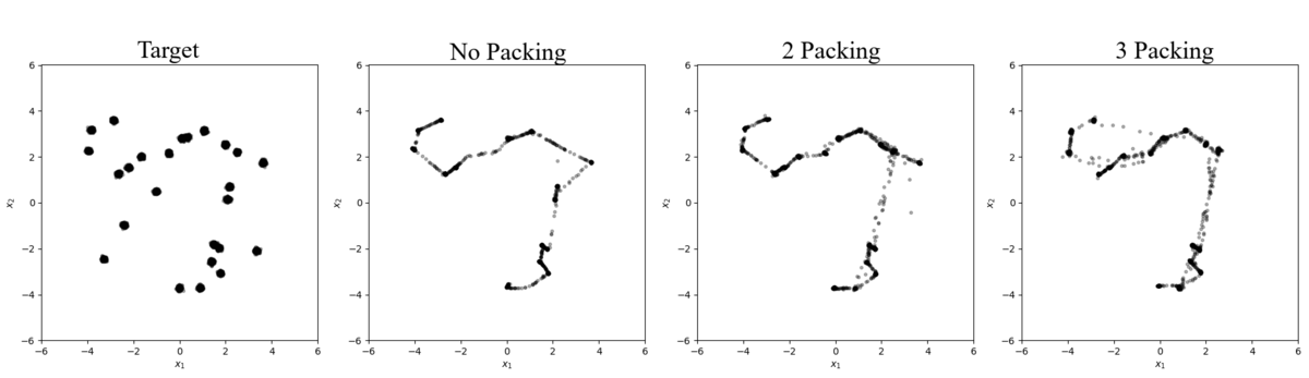
Figure 6: Samples from a 23 randomly spaced mode distribution with $\Sigma=0.0025 \cdot \mathcal{I}$
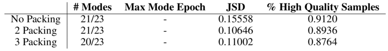
Table 8: Results from Figure 6
Across all experiments, a couple of trends can be seen about packing:
1. As the packing degree $m$ increases, the number of epochs it takes the network to discover all the target distribution’s modes also increases. This is best seen in the experiment with $\Sigma = 0.1 \cdot \mathcal{I}$ (Figure 3 and Table 5) where the network not using packing takes 16 epochs to discover all 25 modes while using packing with $m=2$ takes 27 epochs and $m=3$ takes 62. The reason behind this can be explained by how increasing $m$ causes the discriminator to become stricter about the diversity of the inputs it is validating. This leads to the generator being given less information and as a result taking longer to learn. This is the biggest downfall of packing since GAN training is already very slow and other techniques like adding noise do not hinder the model’s convergence rate to the same degree.
2. Packing is shown to generate a distribution with a smaller JSD compared that from a standard GAN. In some cases, this can be explained simply by the model discovering more modes which cause a lower JSD by definition however this fact can be also observed in experiments where both the packing and non-packing networks discover the same number of modes ($\Sigma = 0.1 \cdot \mathcal{I}$ [Figure 3 and Table 5] and randomly spaced modes [Figure 6 and Table 8]). Since minimizing the JSD is equivalent to finding the optimal discriminator [Goodfellow14], we can say that packing produces a theoretically better model. On the other side, packing has shown to decrease the proportion of high-quality samples compared to that of the standard GAN during these experiments. This quality difference can be explained by how packing causes the network to take more time to discover all the modes (which it is capable of discovering) leading to less time for the generator to prioritize producing high-quality samples. If we were to continue training beyond the 100 epochs done in the experiments, the packing networks should be capable of eventually achieving the same % high-quality samples as the standard GAN.
Using JSD as a model quality metric has also been found to have issues. In image generation, a small JSD has been shown to not always be correlated with visually superior samples and is the reason why models are typically evaluated using metrics like Inception score [Salimans16] or FID [Heusel17]. The advantage of a lower JSD is therefore not as significant as we may have hoped for in image generation but in other domains like numerical data, this may be an important property for a model to have.
Conclusion
Packing is a simple extension to the standard discriminator architecture that empirically shows to reduce mode collapse in many cases. The technique typically produces a distribution that includes more modes from the target distribution with a lower JS divergence than a non-packing network however other techniques like using noise can also alleviate mode collapse while taking less time to train. Packing is an interesting technique that may be beneficial in certain cases but has issues which hold it back from being widely usable.
References
[Goodfellow14] Goodfellow, I., Pouget-Abadie, J., Mirza, M., Xu, B., Warde-Farley, D., Ozair, S., … & Bengio, Y. (2014). Generative adversarial nets. In Advances in neural information processing systems (pp. 2672-2680).
[Lin18] Lin, Z., Khetan, A., Fanti, G., & Oh, S. (2018). Pacgan: The power of two samples in generative adversarial networks. In Advances in Neural Information Processing Systems (pp. 1498-1507).
[Goodfellow13] Goodfellow, I. J., Warde-Farley, D., Mirza, M., Courville, A., & Bengio, Y. (2013). Maxout networks. arXiv preprint arXiv:1302.4389.
[Kingma14] Kingma, D. P., & Ba, J. (2014). Adam: A method for stochastic optimization. arXiv preprint arXiv:1412.6980.
[Arjovsky17] Arjovsky, M., & Bottou, L. (2017). Towards Principled Methods for Training Generative Adversarial Networks. arXiv preprint arXiv:1701.04862.
[Salimans16] Salimans, T., Goodfellow, I., Zaremba, W., Cheung, V., Radford, A., & Chen, X. (2016). Improved techniques for training gans. In Advances in neural information processing systems (pp. 2234-2242).
[Heusel17] Heusel, M., Ramsauer, H., Unterthiner, T., Nessler, B., & Hochreiter, S. (2017). Gans trained by a two time-scale update rule converge to a local nash equilibrium. In Advances in Neural Information Processing Systems (pp. 6626-6637).
[Cho18] Cho, J. (2018, April 04). CycleGAN : Image Translation with GAN (4). Retrieved from http://tmmse.xyz/2018/04/02/image-translation-with-gan-4/
Next
- Training Log Entry 1
Prev -
Belief Contractions on Large Ontologies with Minimal Knowledge Loss