
Belief Contractions on Large Ontologies with Minimal Knowledge Loss
The following was work I did during my NSERC Undergraduate Research Assistant position at Simon Fraser University during Summer 2018. The report assumes the reader has prior knowledge about knowledge representation particularly descriptive logics.
Code can be found here.
The field of knowledge representation deals with finding efficient methods to represent, store and perform inference on large collections of data. When dealing with large knowledge bases, a user may require to remove a fact that was previously believed to be true however has been rendered false after the addition of new information. What makes this operation difficult is that simply removing the belief (represented as a formal logic axiom) is often not enough since the combinations of many other beliefs in the knowledge base can also infer the same false fact resulting in no knowledge actually being removed. Various contraction methods working on different formal logics have been proposed which ensures that a belief is completely forgotten by removing multiple axioms from a knowledge base. In [Dawood17], a kernel contraction algorithm was constructed for $\mathcal{EL}$ TBox. The contraction is performed by removing a minimum set of axioms which infer the belief and using a heuristic to select the a prefered set when multiple minimum sets exist. One of these heuristics is Specificity which weighs axioms by their generality within the domain. We will be expanding upon the Specificity heuristic to create a total preorder relation that orders axioms based on the amount of epistemic loss that they cause when removed from a TBox. The Hierarchical Total Preorder, will work on $\mathcal{EL^{++}}$ TBoxes and will be shown how it can be implemented into the kernel contraction algorithm.
$\mathcal{EL^{++}}$ Description Logic
Description Logics (DL) [Baader07] are a family of logics used to model relationships between entities in a domain. DLs consist of three types of entities, concepts which represent sets of individuals, roles which describe relationships between individuals and singleton individuals from a domain. A DL knowledge base is composed of two parts, the ABox containing extensional knowledge and the TBox containing intensional knowledge. The ABox states assertions about individuals using concepts and roles such as $Doctor(Betty)$ and $brotherOf(Tim, Jill)$. The TBox contains subsumption axioms that describe relationships between concepts and roles such $Dog \sqsubseteq Animal$ and $brotherOf \sqsubseteq parentOf$. Many DLs exist with varying expressibility and reasoning complexity. The language that we will be using is $\mathcal{EL^{++}}$.
$\mathcal{EL^{++}}$ [Baader05], an extension of $\mathcal{EL}$, is a lightweight DL that has limited expressibility but boasts polynomial time reasoning and is used on large ontologies like SNOMED CT. The table below outlines the syntax of the language.
| Name | Syntax | Semantics |
|---|---|---|
| top | $\top$ | $\Delta^{I}$ |
| bottom | $\bot$ | $\emptyset$ |
| nominal | {$a$} | {$a^I$} |
| conjunction | $C \sqcap D$ | $C^I\cap$$D^I$ |
| existential restriction | $\exists r.C$ | {$x \in \Delta^I$ $|$$\exists$ $y \in \Delta^I$: $(x,y) \in$ $r^I$ $\land$ $y$ $\in$ $C^I$} |
| concrete domain | $p(f_1, … ,f_k)$ for $p \in$ $R$ | {$x \in$ $\Delta^I$ $|$$\exists y_1, … , y_k \in$ $\Delta^{D_j}$: $f_i^I(x) = y_i$ for $1 \le i \le k \land$ $(y_1, … y_k)$ $\in p^{D_j}$} |
| GCI | $C \sqsubseteq D$ | $C^I \sqsubseteq D^I$ |
| RI | $r_1 \circ … \circ r_k \sqsubseteq r$ | $r_1^I \circ … \circ r_k^I \sqsubseteq r^I$ |
An $\mathcal{EL^{++}}$ TBox is a finite and consistent set of GCIs and RIs. We refer to the left hand side expression as the sub-concept or sub-role and the right hand side expression as the super-concept or super-role for GCIs and RIs respectively.
Belief Change
The most prominently used construction of belief change is the AGM framework [Alchourron85]. The framework models an agent’s state of knowledge with a belief set which is a closed under logical implication set of sentences. Belief sets state exactly what the agent currently perceives as true. There are three belief change operations for modifying these sets:
- Expansion: Adding a new belief to a belief set.
- Contraction: Removing a belief from a belief set.
- Revision: Adding a new belief which may create an inconsistent belief set that requires other beliefs to be removed.
The operation we will be focusing on is contraction.
While AGM describes contractions using belief sets, [Hansson93] describes a different approach using belief bases. Belief bases are sets of beliefs not closed under logical implication which better models what an agent with finite memory would store and are equivalent to DL TBoxes.
Two methods of belief base contractions are regularly used, partial meet contractions and kernel contractions. Partial meet contractions [Alchourron85] are done by using remainder sets, maximal subsets of a belief base $K$ that do not entail the axiom we wish to contract, $\alpha$. The contracted belief base is the intersection of a select set of remainder sets. Kernels [Hansson94] are minimal subsets of $K$ that entail $\alpha$. To perform a kernel contraction of $\alpha$ we select an axiom from each kernel and remove them from the belief base. Kernel contraction is the method that we will be considering from now on and is denoted by $K \div \alpha$.
The following five postulates [Hansson93] are used to capture the definition of a belief base kernel contraction:
- Success: If $\nvdash \alpha$ then $K\div\alpha \nvdash \alpha$
- Inclusion: $K\div \alpha \subseteq K$
- Core retainment: If $\beta \in K$ and $\beta \notin K\div\alpha$ then there is a set $K’ \subseteq K$ such that $K’ \nvdash \alpha$ but $K’ \cup \beta \vdash \alpha$
- Uniformity: If for every $K’ \subseteq K$ we have$K’ \vdash \alpha$ iff $K’ \vdash \beta$ then $K \div \alpha = K \div \beta$
- Relative closure: $K \cap Cn(K\div\alpha) \subseteq K\div \alpha$
If a function satisfies the first four postulates then it is a kernel contraction and if all five hold then it is a smooth kernel contraction.
The kernel contraction algorithm that we will be working was introduced in [Dawood17]. The algorithm calculates all $\alpha$-kernels, kernels that entail $\alpha$, in $K$ using the axiom pinpointing algorithm [Baader08]. We denote the set of $\alpha$-kernels in belief base $K$ with $K \perp \alpha$. An incision function then selects axioms from each kernel to remove from the belief base. The set of axioms chosen by the incision function is called the drop set, $\sigma(K \perp\alpha)$. Since we prefer to remove as few axioms as possible, the incision function selects a minimum drop set. The calculation for minimum drop sets is equivalent to the minimum hitting set problem [Garey79, Dawood17] therefore a hitting set algorithm is used to find drop sets. Once a minimum hitting set is selected for the drop set, the axioms are removed to form the contracted belief base, $K \div \alpha$.
Hierarchical Total Preorder
Since an $\mathcal{EL^{++}}$ TBox is equivalent to a belief base we can use the kernel contraction $T\div\alpha$ on some $\mathcal{EL^{++}}$ TBox $T$ and axiom $\alpha$. Once the kernels are calculated and the minimum hitting sets are found we typically have multiple equal sized sets to choose as the drop set. Aside from simply removing as few axioms as possible, we ideally want to achieve the contraction with as minimal knowledge loss to the TBox as possible. Expanding on the specificity heuristic from [Dawood17] and exploiting the axiom hierarchy found in $\mathcal{EL^{++}}$, we can define a total preorder binary relation which can order axioms by their importance within the TBox to help make our decision.
The hierarchical preorder relation, $\le_{HP}$, is based off the concept of an epistemic entrenchment [Gardenfors88], $\le_{EE}$. An epistemic entrenchment is a total preorder over the axioms of a belief set that represents the relative epistemic loss caused by removing each axiom. The relation $\alpha \le_{EE} \beta$ states that $\beta$ is equally or more entrenched in the knowledge base as $\alpha$ and therefore during contractions we would prefer to remove $\alpha$ over $\beta$. An epistemic entrenchment is defined by five postulates, transitivity, dominance, conjunctiveness, minimality and maximality. These postulates capture the definition of epistemic loss in standard logics however not all postulates can be applied to description logics.
For the hierarchical preorder, we will form a new set of postulates to formulate a preorder that still uses the metric of epistemic loss to order the axioms but can applied on $\mathcal{EL^{++}}$ TBoxes. In $\mathcal{EL^{++}}$ we can measure epistemic loss as the number of entailments related to the most general expression that are lost. For example, in the TBox $ T =${$A \sqsubseteq B, B \sqsubseteq C, C \sqsubseteq D$}, removing $C \sqsubseteq D$ results in losing the entailments $A \sqsubseteq D, B \sqsubseteq D$ and $C \sqsubseteq D$, however removing $A \sqsubseteq B$ only loses the entailment $A \sqsubseteq D$. Since removing $A \sqsubseteq B$ causes less epistemic loss we have $A \sqsubseteq B \le_{HP} C \sqsubseteq D$.
Before we formulate the postulates we need to first define some terminology that will help us describe the subsumption hierarchy of $\mathcal{EL^{++}}$ axioms.
Def 1 Connected Axioms:
For some TBox $T$ and axioms {$A\sqsubseteq B, C\sqsubseteq D$} $\in T$, where $A,B,C,D$ are either all concepts, existential restrictions and conjunctions (GCI) or all roles (RI). If either:
- {$A\sqsubseteq B, C\sqsubseteq D$}$ \models A\sqsubseteq D$
- {$A\sqsubseteq B, C\sqsubseteq D, \mathcal{S}$}$ \models A\sqsubseteq D$, where $\mathcal{S} \subseteq T$ are support axioms, and no subset of {$A\sqsubseteq B, C\sqsubseteq D, \mathcal{S}$} entails $A\sqsubseteq D$
then $A\sqsubseteq B$ is connected with $C\sqsubseteq D$, $A\sqsubseteq B \mapsto C\sqsubseteq D$. We refer to $A\sqsubseteq B$ as a $\textit{LHS connecting axiom}$ of $C\sqsubseteq D$ and $C\sqsubseteq D$ as a $\textit{RHS connecting axiom}$ of $A\sqsubseteq B$.
Def 2 Subsumption Path:
For some TBox $T$, axioms $\alpha$ and $\beta$ are on the same $\textit{subsumption path}$ if there exists a sequence of axioms {$x_1, x_2, … , x_n$}$\in T$ for $n\geq1$, where both:
- $x_i \mapsto x_{i+1}$ for all $1 \leq i \leq n-1$.
- $x_1 = \alpha$ and $x_n = \beta$.
{$x_1, x_2, … , x_n$} is a $\textit{subsumption path}$ of $\alpha$ and $\beta$.
We now define the four postulates that we will be following while constructing the hierarchical preorder:
- Transitivity: If $\alpha\le_{HP}\beta$ and $\beta \le_{HP}\delta$, then $\alpha \le_{HP}\delta$.
- Totality: For all $\alpha, \beta$, $\alpha \le_{HP} \beta$ or $\beta \le_{HP} \alpha$.
- Minimality: If belief base $T$ is consistent, then $\alpha\notin T$ iff $\alpha \le_{HP}\beta$ for all $\beta$.
- Hierarchical: If $\alpha \mapsto \beta$ and {$\alpha, \beta$}$ \in T$ for some belief base $T$, then $\alpha \le_{HP}\beta$.
Transitivity and totality are the two properties a total preorder must follow. The hierarchical postulate is a new postulate that captures the connection between subsumption hierarchies and epistemic loss in description logics. For example, if we have $\alpha \mapsto \beta$ then$\beta$ is higher in the subsumption hierarchy than $\alpha$ which means removing it will cause more entailments to be lost from the TBox, therefore $\beta$ causes more epistemic loss than $\alpha$.
Hierarchical Weighting Function
When given a hierarchical preorder relation like $\alpha \le_{HP} \beta$, we must determine which of the axioms causes the greater amount of epistemic loss when removed. To measure this, we will weights axioms based on their position within the TBox using the hierarchical weighting function.
The function takes an axiom $\alpha$ and first confirms if $\alpha \in T$ (if not we assign $weight(\alpha) = -1$) and then calculates $weight(\alpha)$ by going through the following 4 phases.
Subsumption Hierarchy Phase
The initial phase weighs $\alpha$ based off its placement within the TBox’s subsumption hierarchy. This is calculated by using the set of LHS connecting axioms of $\alpha$, $LHS(\alpha)$. To find the LHS connecting axioms that appear from using support axioms we first calculate the indirect children of the existential restrictions in the TBox.
Def 3 Indirect Child:
Given $A$ is a concept, existential restriction or a conjunction of concepts and existential restrictions, $B$ and $C$ are concepts and $r$ and $s$ are roles:
- If {$\exists r.C \sqsubseteq A, B\sqsubseteq C$} $\in T$, then $children’(\exists r.C) = children(\exists r.C)\cup${$\exists r.B$}
- If {$\exists r.C \sqsubseteq A, s\sqsubseteq r$} $\in T$, then $children’(\exists r.C) = children(\exists r.C) \cup ${$\exists s.C$}
- If {$\exists r.C \sqsubseteq A, B\sqsubseteq C, s\sqsubseteq r$} $\in T$, then $children’(\exists r.C) = children(\exists r.C)\; \cup $ {$\exists r.B, \exists s.C, \exists s.B$}
We can use these indirect children to find all LHS connecting axioms for each axiom by using the rule:
- $A\sqsubseteq B \in LHS(C\sqsubseteq D)$ if $B = C$ or $B \in children’(C)$
The subsumption hierarchy weighting procedure can now be executed as follows:
Subsumption Hierarchy Weighting Procedure:
- If $LHS(\alpha) = \emptyset$ then $weight(\alpha)=0$.
- If $LHS(\alpha) \ne \emptyset$ then $weight(\alpha) = i+1$ where $i$ is the maximum subsumption hierarchy weight among all axioms in $LHS(\alpha)$.
Since cycles are allowed to occur in the TBox we have an anti-cycling check for the recursive step in the above procedure. While keeping a list of all previously visited axioms in the current recursive stack, if we try to get $weight(\beta)$ and $\beta$ is already in the visited axiom list we do not consider its weight at the current recursion level.
An example of the subsumption hierarchy weightings procedure is shown in the following:
Example 1:
TBox:
| $A \sqsubseteq B $ | $B \sqsubseteq C$ | $C \sqsubseteq \exists r.D$ | $\exists p.E \sqsubseteq F$ |
| $A \sqsubseteq \exists p.E$ | $D \sqsubseteq E$ | $r \sqsubseteq s$ | $s \sqsubseteq p$ |
LHS Connecting Axioms:
| $LHS(A \sqsubseteq B)= \{\} $ | $LHS(B \sqsubseteq C)=\{A \sqsubseteq B \}$ |
| $LHS(C \sqsubseteq \exists r.D)=\{B \sqsubseteq C\}$ | $LHS(\exists p.E \sqsubseteq F)=\{C \sqsubseteq \exists r.D, A \sqsubseteq \exists p.E\}$ |
| $LHS(A \sqsubseteq \exists p.E) =\{\}$ | $LHS(D \sqsubseteq E)=\{\}$ |
| $LHS(r \sqsubseteq s)=\{\} $ | $LHS(s \sqsubseteq p)=\{r \sqsubseteq s\}$ |
Weights:
| $weight(A \sqsubseteq B)=0$ | $weight(B \sqsubseteq C)=1$ |
| $weight(C \sqsubseteq \exists r.D)=2$ | $weight(\exists p.E \sqsubseteq F)=3$ |
| $weight(A \sqsubseteq \exists p.E)=0$ | $weight(D \sqsubseteq E)=0$ |
| $weight(r \sqsubseteq s)=0$ | $weight(s \sqsubseteq p)=1$ |
Support Axiom Phase
An issue with subsumption hierarchy weights is that support axioms are under-weighted. If we consider Example 1, we have $C \sqsubseteq \exists r.D \mapsto \exists p.E \sqsubseteq F$ because of the support axioms $S =${$r \sqsubseteq s, s \sqsubseteq p, D \sqsubseteq E$}. With the axioms of S we have $T \models C \sqsubseteq F$ however if we remove any of these axioms this would not hold. When we perform a contraction of $A \sqsubseteq E$ on TBox T we get 2 kernels:
- $K_1 =$ {$A \sqsubseteq B, B \sqsubseteq C, C \sqsubseteq \exists r.D, \exists p.E \sqsubseteq F, D \sqsubseteq E, r \sqsubseteq s, s \sqsubseteq p$}
- $K_2 = ${$A \sqsubseteq \exists p.E, \exists p.E \sqsubseteq F$}
Removing the lowest weighted axiom in $K_2$ we simply choose $A \sqsubseteq \exists p.E$, however $K_1$ has 3 axioms with a weight of 0 to choose from, $A \sqsubseteq B, r \sqsubseteq s$, and $D \sqsubseteq E$. The issue is removing $A \sqsubseteq B$ preserves $T \models C \sqsubseteq F$, while removing either $r \sqsubseteq s$ or $D \sqsubseteq E$ does not because its causes $C \sqsubseteq \exists r.D \mapsto\mkern-16mu\not \exists p.E \sqsubseteq F$. Since removing these two axioms causes a greater amount epistemic loss to the TBox we need to adjust their weights to reflect this.
The support axiom weighting phase makes adjustments by matching the support axioms’ sub-concept/role with axioms that have existential restrictions with the same concept/role in their super-concept.
Support Axiom Weighting Procedure:
Given $A,B$ are concepts and $r,s$ are roles:
For axioms in the form $A \sqsubseteq B$ with $weight(A \sqsubseteq B) = i$:
- If $X \sqsubseteq \exists r.A \in T$ with $weight(X \sqsubseteq \exists r.A) = j$ and $j \ge i$, then $weight(A \sqsubseteq B) = j$.
For axioms in the form $r \sqsubseteq s$ with $weight(r \sqsubseteq s) = i$:
- If $X \sqsubseteq \exists r.A \in T$ with $weight(X \sqsubseteq \exists r.A) = j$ and $j \ge i$, then $weight(r \sqsubseteq s) = j$.
Continuing with Example 1, applying the support axiom weighting procedure results in the following:
Example 1 cont.
Support Axiom Adjustments:
- Since {$C \sqsubseteq \exists r.D , r \sqsubseteq s$} $\in T$, $weight(C \sqsubseteq \exists r.D) = 2$ and $weight(r \sqsubseteq s) = 0$, set $weight(r \sqsubseteq s) = 2$.
- Since {$C \sqsubseteq \exists r.D , D \sqsubseteq E$} $\in T$, $weight(C \sqsubseteq \exists r.D) = 2$ and $weight(D \sqsubseteq E) = 0$, set $weight(D \sqsubseteq E) = 2$.
Weights:
| $weight(A \sqsubseteq B)=0$ | $weight(B \sqsubseteq C)=1$ |
| $weight(C \sqsubseteq \exists r.D)=2$ | $weight(\exists p.E \sqsubseteq F)=3$ |
| $weight(A \sqsubseteq \exists p.E)=0$ | $weight(D \sqsubseteq E)=2$ |
| $weight(r \sqsubseteq s)=2$ | $weight(s \sqsubseteq p)=1$ |
Cycle Adjustment Phase:
Next is an optional phase to deal with cyclic TBoxes. Say we have the TBox:
| $A \sqsubseteq B$ | $B \sqsubseteq C$ | $C \sqsubseteq A$ |
The weights assigned in the subsumption hierarchy phase varies depending on the order the axioms are processed. For example, if we start with $B \sqsubseteq C$ we would gets the weights:
| $weight(A \sqsubseteq B) = 1$ | $weight(B \sqsubseteq C) = 2$ | $weight(C \sqsubseteq A) = 0$ |
The anti-cycling check prevents the procedure from entering an infinite loop however the hierarchical postulate is broken because $weight(B \sqsubseteq C) > weight(C \sqsubseteq A)$. Another problem is that the current weights state that removing $C \sqsubseteq A$ causes the least amount of epistemic loss however all of the axioms in the loop cause the same amount of loss. To fix both these issues, the cycle adjustment procedure identifies loops and increases all of the loop’s axioms to the maximum weight among these axioms.
Cycle Adjustment Procedure:
- If $\alpha$ is in a cycle comprised of the set of axioms $\ell \subseteq T$, then $weight(\beta) = i$ where $i = max(weight(\beta))$ for all $\beta \in \ell$.
Applying this procedure on the above TBox gives us the weights:
| $weight(A \sqsubseteq B) = 2$ | $weight(B \sqsubseteq C) = 2$ | $weight(C \sqsubseteq A) = 2$ |
Offset Adjustment Phase
The support axiom phase adjusts support axioms’ weights to better reflect their potential epistemic loss within the TBox, however these adjustments can break the hierarchical postulate. In Example 1’s TBox, we currently have $weight(r\sqsubseteq s) = 2$ and $weight(s \sqsubseteq p) = 1$ however since $r \sqsubseteq s \mapsto s \sqsubseteq p$ we require $weight(r \sqsubseteq s) \leq weight(s \sqsubseteq p )$. The offset adjustment procedure fixes this by checking that all of the axioms have a larger weight than their LHS connecting axioms and increases the axiom’s weight when this does not hold.
Offset Adjustment Procedure:
- If $LHS(\alpha) = \emptyset$:
- $o_{\alpha} = 0$
- Else, For all $\beta \in LHS(\alpha)$:
- If $weight(\beta) > weight(\alpha)$, then $o_{\alpha} = o_{\beta} + weight(\beta) - weight(\alpha) +1$
- Else, $o_{\alpha} = o_{\beta}$
- $weight(\alpha) = weight(\alpha) + o_{\alpha}$
Like the subsumption hierarchy weighting procedure, the offset adjustment procedure also contains the same anti-cycling check during the recursive step of calculating $o_{\beta}$ to prevent infinite loops.
Finishing Example 1, we go through the offset adjustment phase and get the following:
Example 1 cont.
Offset Adjustments:
- Since $weight(r \sqsubseteq s) > weight(s \sqsubseteq p )$:
- $o_{s \sqsubseteq p} = o_{r \sqsubseteq s} + weight(r \sqsubseteq s) - weight(s \sqsubseteq p) +1 = 0 + 2 - 1 + 1 = 2$
- $weight(s \sqsubseteq p) = 1 + 2 = 3$.
Weights:
| $weight(A \sqsubseteq B)=0$ | $weight(B \sqsubseteq C)=1$ |
| $weight(C \sqsubseteq \exists r.D)=2$ | $weight(\exists p.E \sqsubseteq F)=3$ |
| $weight(A \sqsubseteq \exists p.E)=0$ | $weight(D \sqsubseteq E)=2$ |
| $weight(r \sqsubseteq s)=2$ | $weight(s \sqsubseteq p)=3$ |
Using Hierarchical Weighting Function in $\le_{HP}$
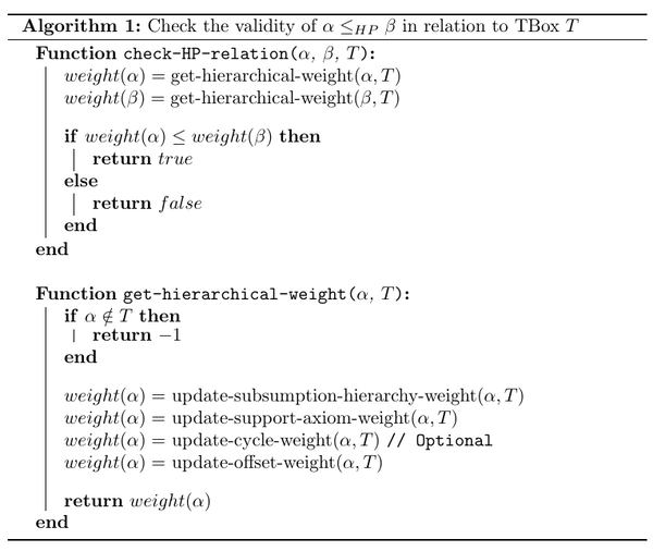
With the hierarchical weighting function we can now implement $\le_{HP}$ to solve hierarchical preorder relations using the following rule:
- $\alpha \le_{HP} \beta$ iff $weight(\alpha) \le weight(\beta)$
Algorithm 1 outlines the relation validity checking and weight calculation processes. Here we are assuming that the TBox T stores pairs of axioms and their weights.
Postulate Proofs
We will now prove that the hierarchical preorder relation follows the postulates previously introduced.
Theorem: The hierarchical preorder binary relation $\le_{HP}$ satisfies the transitivity, totality, minimality and hierarchical postulates when applied to an EL++ TBox.
Proof: Given TBox $T$ and axioms $\alpha, \beta,\delta$.
Transitivity: Assume $\alpha \le_{HP} \beta$ and $\beta \le_{HP} \delta$. This means that $weight(\alpha) \le weight(\beta)$ and $weight(\beta) \le weight(\delta)$ which implies $weight(\alpha) \le weight(\delta)$ therefore giving $\alpha \le_{HP} \delta$.
Totality: For all $\alpha, \beta$ we have their weights, $weight(\alpha)$ and $weight(\beta)$. If $weight(\alpha) \le weight(\beta)$ then $\alpha \le_{HP} \beta$ and if $weight(\beta) \le weight(\alpha)$ then $\beta \le_{HP} \alpha$. Therefore for all $\alpha, \beta$, we have $\alpha \le_{HP} \beta$ or $\beta \le_{HP} \alpha$
Minimality: ($\Longrightarrow$) Assume T is consistent and $\alpha \notin T$. In the hierarchical weighting function we initially check if $\alpha \in T$. Since this is false, we assign $weight(\alpha) = -1$. The minimum weight any axiom $\beta$ can have is -1, therefore $weight(\alpha) \le weight(\beta)$ and $\alpha \le_{HP} \beta$ for all $\beta$.
($\Longleftarrow$) Assume T is consistent and $\alpha \le_{HP} \beta$ for all $\beta$. We then get $weight(\alpha) \le weight(\beta)$ for all $\beta$. Since $T$ is consistent, we know that there exists some axiom $\delta \notin T$ that would make $T$ inconsistent, therefore $weight(\delta) = -1$. Since $weight(\alpha) \le weight(\beta)$ for all $\beta$ we must have $weight(\alpha)=-1$ which can only occur when $\alpha \notin T$.
Hierarchical: Assume $\alpha \mapsto \beta$ and ${\alpha,\beta} \in T$. To check if $\alpha \le_{HP}\beta$ we begin by getting $weight(\alpha)$ and $weight(\beta)$. At the start of offset adjustment phase we have $weight(\alpha) = i$ and $weight(\beta) = j$ where $i,j \ge 0$. During the phase, offsets for $\alpha$ and $\beta$, $o_{\alpha}$ and $o_{\beta}$, are calculated and added to each of the axioms’ weights. Depending on the values of $i$ and $j$, $o_{\beta}$ has the value:
- If $i>j$ then $o_{\beta} = o_{\alpha}+i-j+1$
- If i $\le$ j then $o_{\beta} = o_{\alpha}$
Applying these offsets, we get:
- If $i>J$:
$$ \begin{aligned} weight(\alpha) &= i + o_{\alpha} \\ weight(\beta) &= j + o_{\beta} \\ &= j + o_{\alpha} +i - j + 1 \\ &= i + o_{\alpha} +1 \end{aligned} $$
- If $i \le j$:
$$ \begin{aligned} weight(\alpha) &= i + o_{\alpha} \\ weight(\beta) &= j + o_{\beta} \\ &= i + o_{\alpha} \end{aligned} $$
Therefore the hierarchical weighting function always terminates with $weight(\alpha) \le weight(\beta)$ and thus always returns $\alpha \le_{HP} \beta$ whenever $\alpha \mapsto \beta$ and ${\alpha, \beta} \in T$.
This proves that the hierarchical preorder binary relation $\le_{HP}$ satisfies all four postulates.
Kernel Contraction with Hierarchical Preorder
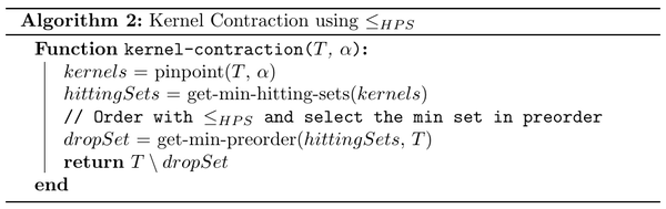
Returning to the problem of selecting which hitting set to remove in the kernel contraction algorithm, we can extend the definition of $\le_{HP}$ to create a new total preorder relation that works with sets of axioms, $\le_{HPS}$. The relation $H_1 \le_{HPS} H_2$ where $H_1,H_2 \subseteq T$ states removing $H_2$ causes an equal or greater amount of epistemic lost as removing $H_1$. For set weights can say $weight(H_1) = sum(weight(\alpha))$ for all axioms $\alpha \in H_1$. To validate $\le_{HPS}$ relations we use the rule:
- $H_1 \le_{HPS} H_2$ if $weight(H_1) < weight(H_2) $ where $H_1, H_2 \subseteq T$
In order for the kernel contraction algorithm to be smooth, we must ensure that the same drop set is chosen every time we repeat a contraction. Therefore we assume that a canonical ordering of the axioms exists which can be used in tiebreakers where multiple axioms have the same minimum weight.
When choosing which hitting set to remove, all of the hitting sets are ordered with $\le_{HPS}$ and then the set that is at the bottom of the preorder is selected as the drop set. Algorithm 2 outlines the kernel contraction algorithm $T\div\alpha$ using $\le_{HPS}$.
Smooth Kernel Contraction Proof
We will now show that $T\div\alpha$ is a smooth kernel contraction by proving that all five postulates hold.
Theorem 2: The kernel contraction described in Algorithm 2 satisfies all five smooth kernel contraction postulates when applied an $\mathcal{EL^{++}}$ TBox.
Proof: Given a TBox $T$ and axioms ${\alpha, \beta}$
Success: Assume $\nvdash\alpha$. When the pinpointing algorithm is applied, a finite number of $\alpha$-kernels are calculated that each entail $\alpha$. $\sigma(T \perp \alpha)$ is a minimum hitting set of the kernels so the set will include axioms from every kernel. Therefore the contracted TBox $T \setminus \sigma(T \perp \alpha)$ will have no $\alpha$-kernels and $T\div\alpha \nvdash \alpha$.
Inclusion: The algorithm never adds new axioms to $T$ therefore $T\div\alpha \subseteq T$.
Core Retainment: Assume $\beta \in T$ and $\beta \notin T\div\alpha$. That means $\beta \in \sigma(T \perp \alpha)$. Set $T’=T-\alpha$ which means $T’ \subseteq T$ and $T’ \nvdash \alpha$. If we add $\beta$ to $T’$ then at least one $\alpha$-kernel exists in $T’ \cup \beta$ since $\beta$ is in a minimal hitting set of the kernels. Therefore $T’ \cup \beta \vdash \alpha$.
Uniformity: Assume for every $T’ \subseteq T$, we have $T’ \vdash \alpha$ iff $T’ \vdash \beta$. In [Hansson94], it is explained that our assumption is equivalent to $T \perp \alpha = T \perp \beta$. When the incision function is run on $T \perp \alpha$ and $T \perp \beta$, the same set of hitting sets will be calculated and since the preorder using $\le_{HPS}$ is unique (assuming $<_*$ exists), $\sigma(T \perp \alpha) = \sigma(T \perp \beta)$ and therefore $T\div\alpha = T\div\beta$.
Relative Closure: For some axiom $\beta$, if $\beta \in T$ and $\beta \in T\div\alpha$, then trivially $\beta \in T \cap Cn(T\div\alpha)$. Also trivially, if $\beta \notin T$ then $\beta \notin T \cap Cn(T\div\alpha)$.
For the case where $\beta \in T$ and $\beta \notin T\div\alpha$. Let us assume that $\beta \in Cn(T\div\alpha)$. We know that $\beta \in \sigma(T \perp \alpha)$ therefore $\beta$ is found in at least one $\alpha$-kernel. More specifically, since all hitting sets calculated are minimum, we know that for all $\alpha$-kernels that contain $\beta$, there must be some $\alpha$-kernel $k$ where no other $\delta \in \sigma(T \perp \alpha)$ is found. If this is not true then the hitting set would not be minimal since $\beta$ would be unnecessary. After removing the axioms of $\sigma(T \perp \alpha)$, we should have contracted $\alpha$ and have $T \perp \alpha = \emptyset$ however since $\beta \in Cn(T\div\alpha)$, there exists a subset of axioms $S \subseteq T\div\alpha$ where $S \vdash \beta$ and therefore $S \cup k \setminus \beta \vdash \alpha$. This contradicts the success postulate for kernel contractions. Therefore $\beta \notin Cn(T\div\alpha)$ thus $\beta \notin T \cap Cn(T\div\alpha)$. Since all axioms fall into one of these cases, we have $T \cap Cn(T\div\alpha) \subseteq T\div \alpha$ always holds.
This proves that Algorithm 2 is a smooth kernel contraction.
Future Work
The hierarchical total preorder relation is a versatile method for ordering axioms and sets of axioms in TBoxes that do not need to be normalized and can be cyclic. When used in kernel contractions, the preorder limits the amount of epistemic loss caused to the TBox and maintains the smooth kernel contraction property.
This hierarchical approach is simply one way of ordering axioms. Future work can be done into developing new preorders or epistemic entrenchments that use different approaches to weighting axioms that work better under certain contexts. An issue with the hierarchical weighting function currently is that after every contraction, the entire TBox needs to be re-weighted in order to update the preorder. Developing a way to adjust weights after a contraction is an avenue to explore further. Finally, though the preorder was construction for $\mathcal{EL^{++}}$ TBoxes, it would be interesting to see if the method can be expanded to work with more expressive descriptions logics like the $\mathcal{ALC}$ family.
References
[Alchourron85] Alchourrón, C., Gärdenfors, P., and Makinson, D. (1985). On the logic of theory change: Partial meet contraction and revi- sion functions. 50(2):510–530.
[Baader05] Baader, F., Brandt, S., and Lutz, C. (2005). Pushing the EL envelope. In Proceedings of the Nineteenth International Joint Confer- ence on Artificial Intelligence IJCAI-05, Edinburgh, UK. Morgan-Kaufmann Publishers.
[Baader07] Baader, F., Calvanese, D., McGuiness, D., Nardi, D., and Patel-Schneider, P., editors (2007). The Description Logic Handbook. Cam- bridge University Press, Cambridge, second edition.
[Baader08] Baader, F. and Suntisrivaraporn, B. (2008). Debugging SNOMED CT using axiom pinpointing in the description logic EL+ . In Proceedings of the 3rd Knowledge Representation in Medicine (KR-MED’08): Representing and Sharing Knowledge Using SNOMED, vol- ume 410 of CEUR-WS.
[Dawood17] Dawood, A., Delgrande, J., and Liao, Z. (2017). A study of kernel contraction in EL. In Gordon, A., Miller, R., and Turan, G., editors, Thirteenth International Symposium on Logical Formalizations of Common- sense Reasoning, London, UK. (7 double-column AAAI-style pages).
[Gardenfors88] Gärdenfors, P. and Makinson, D. (1988). Re- visions of knowledge systems using epistemic entrenchment. In Proceedings of the 2Nd Conference on Theoretical Aspects of Reasoning About Knowl- edge, TARK ’88, pages 83–95, San Francisco, CA, USA. Morgan Kaufmann Publishers Inc.
[Garey79] Garey, M. and Johnson, D. (1979). Computers and Intractability: A Guide to the Theory of NP-Completeness. W.H. Freeman and Co., New York.
[Hansson93] Hansson, S. O. (1993). Reversing the levi identity. 22(6):637– 669.
[Hansson94] Hansson, S. O. (1994). Kernel contraction. 59(3):845–859.
Next
- An Empirical Analysis Packing Discriminators in Generative Adversarial Networks